The appropriate interpretation of the statistical results is crucial to understand the advances in medical science. The statistical tools allow us to transform the uncertainty and apparent chaos in nature to measurable parameters which are applicable to our clinical practice. The importance of understanding the meaning and actual extent of these instruments is essential for researchers, the funders of research and for professionals who require a permanent update based on good evidence and supports to decision making. Various aspects of the designs, results and statistical analysis are reviewed, trying to facilitate his comprehension from the basics to what is most common but no better understood, and bringing a constructive, non-exhaustive but realistic look.
La interpretación de los resultados estadísticos es un elemento crucial para la comprensión de los avances en las ciencias médicas. Las herramientas que nos ofrece la estadística nos permiten transformar la incertidumbre y aparente caos de la naturaleza en parámetros medibles y aplicables a nuestra práctica clínica. La importancia de entender el significado y alcance real de estos instrumentos es fundamental para el investigador, para los financiadores de las investigaciones y para los profesionales que precisan de una actualización permanente basada en buena evidencia y ayudas a la toma de decisiones. Se repasan diversos aspectos de los diseños, resultados y análisis estadísticos, intentando facilitar su entendimiento desde lo más elemental a aquello que es más común pero no por ello mejor comprendido y aportar una mirada constructiva y realista, sin ser exhaustiva.
Clinical research is an indispensable means for the advancement of scientific knowledge and to implement it into the routine clinical practice in order to provide the patients with the best opportunities to recover or improve their health understood as years and quality of life.1
But to accomplish this we are going to need tools to be able to conduct research, describe the biological reality, facilitate the understanding of clinical research and allow manipulation through experiments in order to establish associations between stimuli (drugs, surgical technique, etc.) and interesting results.
Statistical techniques are mathematical models that require certain knowledge for their interpretation.2,3 Without an adequate understanding, the generalization of the study results can be useless or dangerous. From an ethical point of view4 making the effort of trying to understand is essential if we wish to be updated on scientific advances.4 Also, given the huge scientific production available today fueled by the need for publishing to be promoted professionally, it is essential to know how to interpret statistical results in order to distinguish the important stuff from the unimportant one, develop an analytical spirit,5 and assess any possible implications to our clinical and research practice.
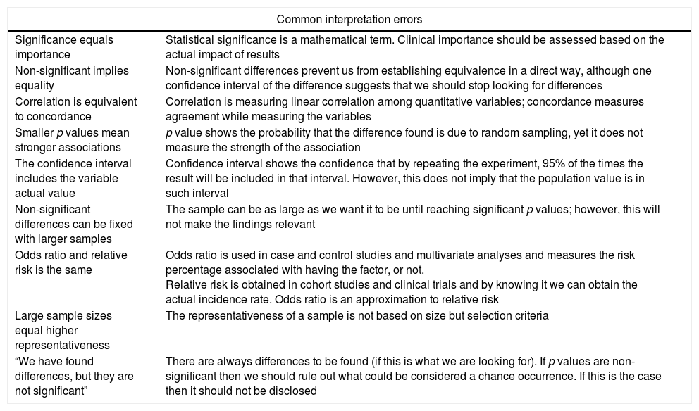
The goal of this study is to provide a general standpoint on the interpretation of the most common statistical results and emphasize all limitations and potential errors (Table 1) for the adequate understanding of such results. Information can be more basic or more complex, not very thorough, but it is always necessary and will always be referenced to its use in the clinical research of the critically ill patient.
Common errors when interpreting statistical results.
| Common interpretation errors | |
|---|---|
| Significance equals importance | Statistical significance is a mathematical term. Clinical importance should be assessed based on the actual impact of results |
| Non-significant implies equality | Non-significant differences prevent us from establishing equivalence in a direct way, although one confidence interval of the difference suggests that we should stop looking for differences |
| Correlation is equivalent to concordance | Correlation is measuring linear correlation among quantitative variables; concordance measures agreement while measuring the variables |
| Smaller p values mean stronger associations | p value shows the probability that the difference found is due to random sampling, yet it does not measure the strength of the association |
| The confidence interval includes the variable actual value | Confidence interval shows the confidence that by repeating the experiment, 95% of the times the result will be included in that interval. However, this does not imply that the population value is in such interval |
| Non-significant differences can be fixed with larger samples | The sample can be as large as we want it to be until reaching significant p values; however, this will not make the findings relevant |
| Odds ratio and relative risk is the same | Odds ratio is used in case and control studies and multivariate analyses and measures the risk percentage associated with having the factor, or not. Relative risk is obtained in cohort studies and clinical trials and by knowing it we can obtain the actual incidence rate. Odds ratio is an approximation to relative risk |
| Large sample sizes equal higher representativeness | The representativeness of a sample is not based on size but selection criteria |
| “We have found differences, but they are not significant” | There are always differences to be found (if this is what we are looking for). If p values are non-significant then we should rule out what could be considered a chance occurrence. If this is the case then it should not be disclosed |
Summary statistics allow us to visualize the characteristics of data distribution by synthesizing the dimension of a variable change, and they are basic concepts in statistics. The arithmetic mean is the sum of each value divided by the total number of individuals from a given population. It is affected by the existence of extreme values, so it is not appropriate for not very uniform distributions,6 such as ICU stays. The trimmed mean eliminates extreme values, and the mode corresponds to the most common value within distribution; however, the utility of both is limited.
Variance is one indicator used to establish the degree of separation of one array (a dataset) with respect to its arithmetic mean, although we normally use the standard deviation (SD) as the square root of the variance expressed in the same units of the variable.7 The SD shows the dispersion of distribution, being one SD above average usually indicative of asymmetrical distribution (when the number of cases is higher in high or low values, such as the ICU stay). If distribution is normal, it will show values where we find 68% (±1SD), 95% (±2SD), or 99.7% (±3SD) of data. This is the origin of the popular expression mean±SD although the term mean (SD) is preferred here.
When the distribution of the variable is asymmetrical we use measures based on order. The mean is the main value obtained after ordering the values. Quartiles, deciles or percentiles are the result of dividing the ordered sample into 4, 10, or 100 equal parts. The mean matches the 2nd quartile, the 5th decile, and the 50th percentile. In these cases, the preferred dispersion means are percentiles 25 and 75 or the difference between the two—called interquartile range (IQR). It is not the same as the range of a variable, indicative of the upper and lower limits of a variable. The ICU stay or the days on mechanical ventilation are values of asymmetrical distribution that we rather express using means and percentiles 25–75 or the IQR.8
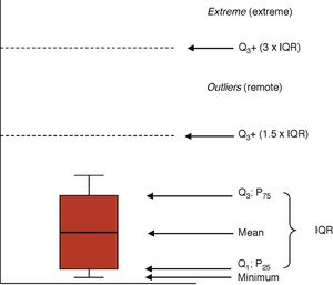
Graphic representationsThe distributions of the quantitative variables are usually represented through histograms (bar diagrams), or dispersion charts (scatter plot). Boxplots (Fig. 1) are highly indicative of the distribution of one variable. The box is limited from the bottom up by quartiles Q1 and Q3 with the mean at the center. The wings of the box contain even the lowest smaller value and the limit of Q3 by at least 1.5 times the IQR. Values above this margin are remote values (above Q3+1.5×IQR) and extreme values (above Q3+3×IQR).
Prevalence and incidencePrevalence is the proportion of cases of a given population showing a particular trait or disease. Prevalence can be point prevalence or period prevalence, when a time-lapse from t0 to t1 is analyzed and the population counted in the middle of an interval. The ENVIN-UCI registry studies are an example of the latter type of design.9 Prevalence studies assess global trends and allow us to generate hypotheses, but not causal relationships.
Incidence is the number of new cases of a given disease or trait in a population throughout a period of time. Cumulative incidence is the proportion of patients at risk who are disease-free in a given period of time. The incidence rate (also called incidence density [ID]) is the number of new cases in a given period of time divided by the sum of time units at risk for every one of the individuals exposed.
For example, in a population of 200 critically ill patients intubated for at least al 48h there are 16 ventilator-associated pneumonias (VAP) throughout a one-month period. The risk or cumulative incidence of VAP will be 16/200=8% for every individual, or 8 for every 100 patients ventilated monthly. In critically ill patients, measuring cumulative incidence can be poorly informative because the risk factors change and there are losses (deceased patients or patients who stop having the risk factor, such as mechanical ventilation). In this case, we can use the actuarial model that takes these losses into consideration, or the ID. The latter is the indicator we use for device-related infections (mechanical ventilation, catheters). It is measured in reciprocal time units (6 VAPs for every 1000 patients per day on mechanical ventilation, 3 catheter-related infections for every 1000 patients per day wearing the catheter). The assessment of risk-related time units can be very important because this does not add cumulative effects caused by maintaining the factors. It is not the same 500 patients spending 3 days on mechanical ventilation than 300 patients spending 5 days, and it is not the same one patient with several catheters and a total of 6 lumens that a patient with a double-lumen catheter even if denominators are the same. By agreement, the total sum of days spent on mechanical ventilation and the total sum of days wearing a catheter are the ones taken into consideration here.10
Measures of associationMeasures of association quantify the existing relation between 2 different variables. Their goal is to establish whether there is an actual association between exposure or trait and a given condition or disease, although this does not presuppose causality. These measures establish whether the frequency of a feature (disease) is different among patients exposed to a given variable.
Absolute percent difference. Also known as risk difference, attributable risk, excess risk, or absolute risk reduction. It shows how increased or decreased the risk of a given event is based on the event group. It is an absolute measure that provides limited information, because a 1% reduction can be very important when basal risk is 2%, but insignificant when the initial risk is as high as 30%.
Disease odds ratio. Odds is a term used in gambling and it shows what the chances are of getting this or that result. For example, if a patient's probability of survival is 75%, and his probability of dying is 25%, the odds of survival would be 75%/25%, or 3-1, or just 3 to simplify. This means that the patient's probability of survival is three times higher than his probability of dying.
Relative percent difference. Also called relative risk difference (RRD), or relative risk reduction (RRR). It is the risk or incidence difference divided by the incidence in the comparison group. It shows how much the risk of changing the comparison group actually varies. It is used to calculate the effect size. For example, going from a 0.99% incidence rate to a 0.75% incidence rate can be more or less clinically relevant, but a 24% relative risk reduction (same data) is much more impressive, especially if the confidence interval of such estimate is not included.11
Proportion ratio. Also called relative risk, or risk rate (RR). It is the most successful indicator of all, and it is estimated as the incidence ratio of the exposed group versus the incidence ration of the non-exposed. It is interpreted as the number of times the risk of having an event is increased o reduced based on exposure. RR>1 is indicative of higher risk; null effect when equal to 1; RR<1 is indicative of lower risk. Since this is a relative measure, it should be accompanied by the absolute incidence data so that the clinical relevance of the effect can be estimated. Mortality rates of 0.03% versus mortality rates of 0.01% would generate a RR=3. On the other hand, the clinical impact of this association might be irrelevant. RR<1 can be difficult to interpret. RR=0.20 is not indicative of a 20% risk reduction but it is indicative of 1/0.20 – a risk that is 5 times lower.
Longitudinal studies and clinical trials use one statistical concept known as number needed to treat (NNT). It tells us how many individuals would need to be treated to achieve an additional positive result or avoid a negative one. It is estimated using the inverse of the absolute difference of incidences.
Odds ratio. Its interpretation depends on the context of the study design where it is used. In case and control studies, the actual incidence rate of the disease in the non-exposed group is unknown because no follow-up of the entire population is conducted, instead one representative sample of this population is selected. With this it is impossible to know the actual RR since we do not have the incidence rate of the non-exposed. However, we can know the odds of exposure to the risk factor in the exposed and non-exposed groups; that is, the highest odds for a patient to be exposed and the highest odds for a non-patient to be exposed. This odds ratio is what we call OR in case and control studies. Its interpretation is an estimate of the incidence ratio in the original population provided that the selection of controls happened independently from the exposure.
Confidence intervalsAll measures taken in a sample of subjects is an estimate of the actual measure in the general population, which is what we wish to know. Whenever we pick a sample, we want it to be representative of the population, which is why we use inclusion and exclusion criteria that facilitate conducting a certain study and do not generate excessive differences with the target population, so we can generalize the results.
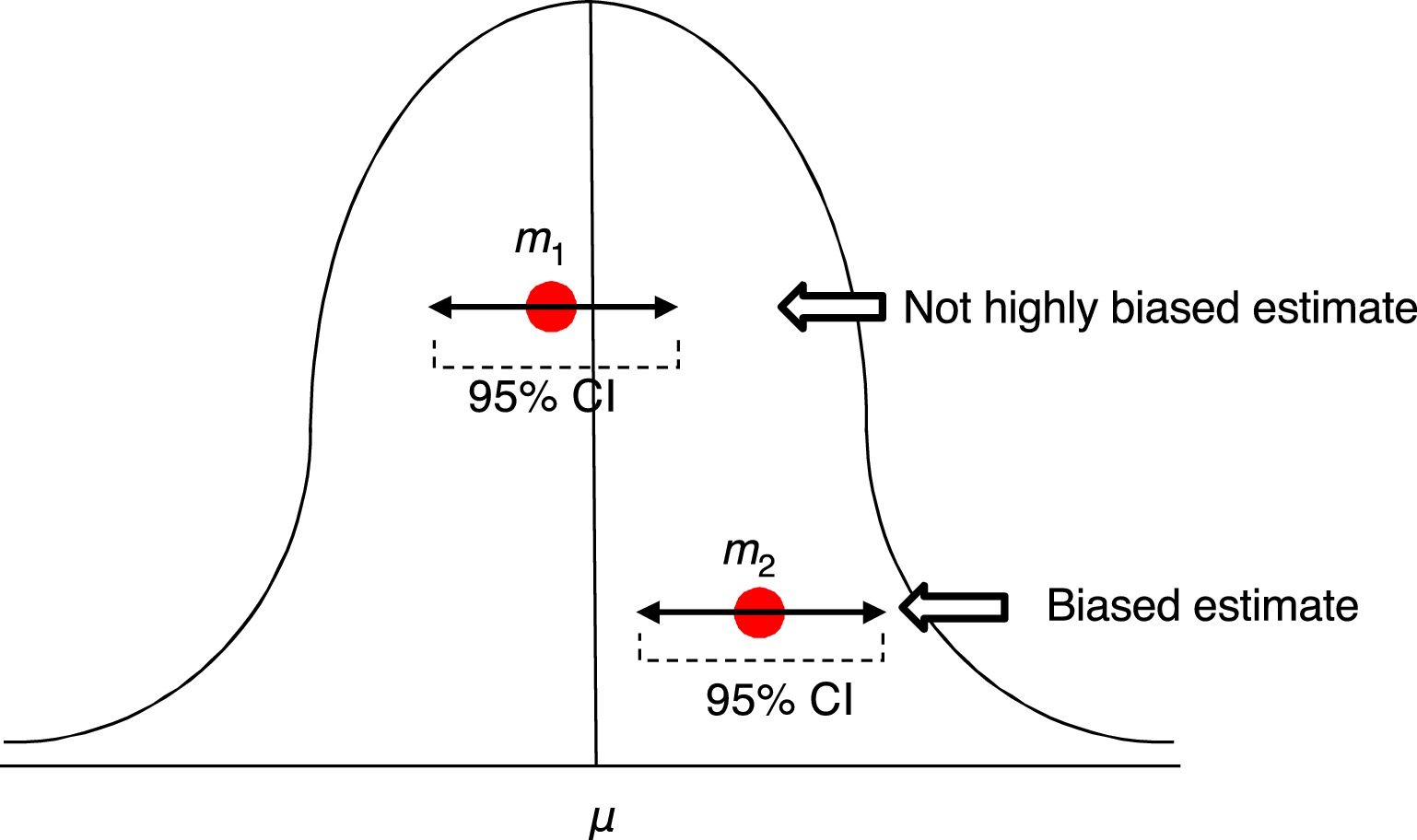
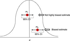
In order to assess the estimate of a measure we use confidence intervals (CI) usually at 95%. Ninety-five percent (95%) CIs does not mean that there is a 95% chance of finding that measure, in that interval, in the actual population. A ninety-five percent (95%) CI means that we are confident that the method used will give us samples that, in 95% of the cases, should generate an estimator included in that interval. But this does not imply that in the actual population the indicator is included in that interval. It may or may not be included (Fig. 2).
Estimates of one mean and its confidence interval at 95%. The first m1 is not a highly biased estimate, while the second m2 is biased, and its confidence interval tells us, with a 95% confidence, that if we repeat the experiment, we will be getting an estimator in such interval that will not include that of the actual μ mean.
Linear regression is the procedure we use to establish a linear correlation (y=a+bx) in the behavior of 2 variables. This can graphically be seen whenever a cloud of dots generated with the pairs of variables comes close to a straight line, which will help us define the values of one variable based on the other one.
Correlation is the linear association between 2 independent variables and is established as an asymmetry in the behavior of both. It is important to emphasize that correlations do not imply the existence of causality, but that there is some sort of association with an intermediate variable between the two.12
In order to measure the correlation between 2 variables we use covariance or its standardization, that is, the Pearson's r correlation coefficient. This index requires a normal distribution of the variables and varies between −1 (negative correlation) and +1 (positive correlation). Whenever its value is close to 0, there is no linear correlation. In cases where distribution is not normal we can use the Spearman or Kendall's rank correlation coefficients to find non-linear correlations.
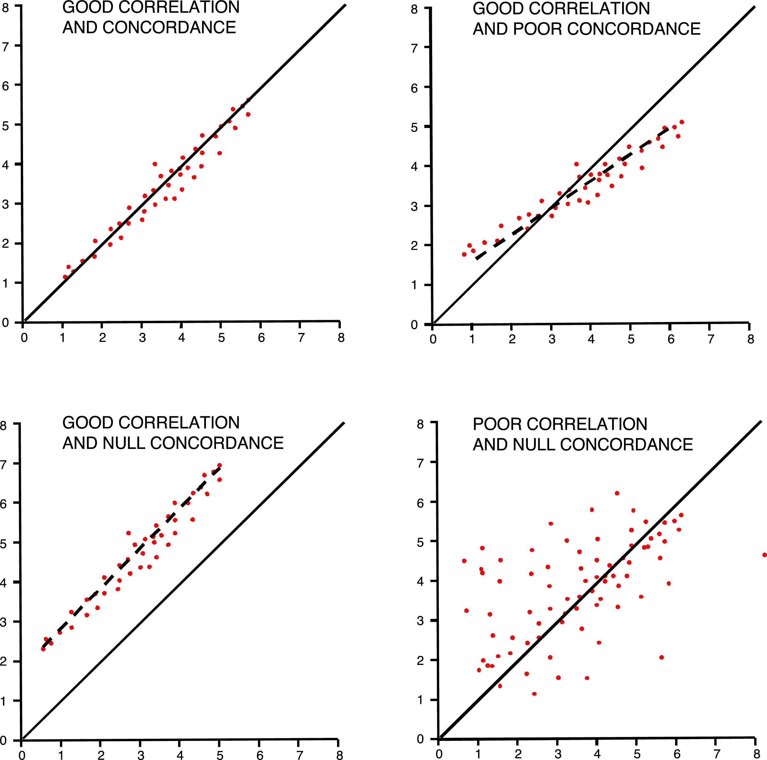
In order to interpret correlations, we should not forget that the Pearson's r coefficient measures the linear correlation, but we can also have non-linear correlations among different variables. It is important to have unbiased measures and check the impact of extreme values. Correlations should have a certain logic when creating the association, avoiding spurious associations, part-whole relationships (APACHE II with renal dysfunction), or variables with estimated values (pH and base excess). Correlations are also commonly and incorrectly used as concordance analyses among different tools for the measurement of one variable.
Reliability studies analyze variation when measuring one variable using one measurement tool and the same observer (intra-observer) or several observers (inter-observer) or concordance between two measurement tools.13 These studies are common in critical care medicine and they estimate invasive parameters through non-invasive means. Concordance among different measures in qualitative variables use the kappa index that measures the inter-rater agreement by subtracting the possibility of the agreement occurring by chance. It fluctuates between 1 (maximum concordance) and values that can be negative. It is estimated that kappa index values >0.6 are indicative of good concordance, and values <0.4 suggest weak concordances. In the case of ordinal or polychotomous variables (e.g. degrees of heart failure), the weighted kappa index is used.14 The kappa index should not be used in qualitative groups of quantitative variables.
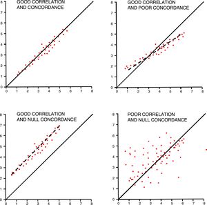
Concordance among quantitative variables measures the interclass correlation coefficient (ICC) that analyzes the variance of subjects, the measurement tool, and the errors made while measuring.15 It has been agreed that good concordances should be over 0.75. One graphic and easy way to check concordance in quantitative variables is the Bland–Altman plot that shows individual differences between measures and their relation to their mean.16 We should not forget that, in these studies, even though it may coincide with the ICC, correlation is not a good method of analysis (Fig. 3).
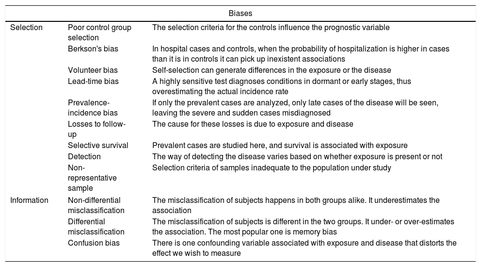
Validity and accuracy of studiesIn a study, validity can be defined as the internal and external consistency of results. This generates confidence that the data obtained are representative of the reality that we wish to observe. If we are conducting a study on critically ill patients with sepsis and we are using criteria of sepsis that have not been updated, then the consistency of results is compromised and, as a result, internal validity. If immunocompromised patients are not included, then the sample may not be representative of the overall population of patients with sepsis, which would compromise external validity. Internal validity is an indispensable prerequisite of a study, and external validity gives us the possibility of generalizing the results obtained. Also, we should be cautious of selection biases (Table 2). One of these biases is considering the critically ill patient as a patient of a certain type and not as a clinical situation per se occurring in different diseases. We can have information biases due to the different number of registries between the ICU and prior admissions, which can generate issues when assessing the variables of interest among patients with different prior ICU stays.17
Common biases in clinical research.
| Biases | ||
|---|---|---|
| Selection | Poor control group selection | The selection criteria for the controls influence the prognostic variable |
| Berkson's bias | In hospital cases and controls, when the probability of hospitalization is higher in cases than it is in controls it can pick up inexistent associations | |
| Volunteer bias | Self-selection can generate differences in the exposure or the disease | |
| Lead-time bias | A highly sensitive test diagnoses conditions in dormant or early stages, thus overestimating the actual incidence rate | |
| Prevalence-incidence bias | If only the prevalent cases are analyzed, only late cases of the disease will be seen, leaving the severe and sudden cases misdiagnosed | |
| Losses to follow-up | The cause for these losses is due to exposure and disease | |
| Selective survival | Prevalent cases are studied here, and survival is associated with exposure | |
| Detection | The way of detecting the disease varies based on whether exposure is present or not | |
| Non-representative sample | Selection criteria of samples inadequate to the population under study | |
| Information | Non-differential misclassification | The misclassification of subjects happens in both groups alike. It underestimates the association |
| Differential misclassification | The misclassification of subjects is different in the two groups. It under- or over-estimates the association. The most popular one is memory bias | |
| Confusion bias | There is one confounding variable associated with exposure and disease that distorts the effect we wish to measure | |
The accuracy of a study is the margin of error with which results have been obtained. It basically depends on the size of the sample, but not exclusively on this. There are registry designs and modes and effective analyses we can use to be more accurate, such as quantitative variables instead of qualitative variables, or conducting survival analyses instead of analyzing the result as one dichotomous variable.
Statistical significance testsStatistical significance tests became popular with Fisher who used the Bayesian approach to propose the following analytical model: considering one null hypothesis H0 (no differences between 2 treatments) as true, an experiment that will provide certain results is conducted and then the p probability is estimated as if H0 were true. A very small p value we would make us look for alternatives to H0, although it would not automatically reject it.
Almost at the same time, Neyman and Pearson proposed an alternative method based on the existence of two (2) hypotheses—the null hypothesis H0 (no differences between 2 treatments), and the alternative H1 (there are some differences)—and type-I errors (made when considering H1 valid when H0 is true) and type-II errors (made when considering H0 valid when H1 is true). The goal of the experiment was to choose between the two based on the probability of making type-I errors (α risk) or type-II errors (β risk).
Today we use one combined method18 by defining one null hypothesis H0 and planning an experiment to detect some difference. Then the p probability of having obtained such results is estimated considering H0 as true. If the p value is small, then the validity of H0 will be rejected (that is, there are no differences), but if it is not, it won’t be, but it will not be accepted either. This means that the lack of statistical significance in a trial is not interpreted as therapeutic equivalence.19
The researchers’ ultimate obsession of obtaining p<0.0520 is based on a general consensus on the Fisher's exact test21 that tries to solve whether a result occurring by chance no more than 1 time per every 20 trials could be considered statistically significant. However, the wanted p value depends on the size of the sample rather than the size of the difference, so all we would need is have larger samples in order to obtain “statistically significant” results.22 It is the responsibility of the researcher to interpret whether a result that is statistically significant can also be considered clinically relevant.23,24 A paper recently published in the NEJM that studied 49,331 urgent admissions due to sepsis25 statistically shows that the risk of hospital mortality goes up 4% every hour (OR 1.04 [95%CI: 1.02–1.05]; p<0.001) when certain measures have not been implemented (hemocultures, antibiotic therapy, and fluids) within a 3-hour window of opportunity. The comparative table shows how the difference between implementing the aforementioned measures within 3h or between 3 and 12h increases mortality rate from 22.6% to 23.6%. These percentages would not be interpreted as different in any other study with a reasonable number of patients, but here they are given a significant p value thanks to the huge size of the sample. It is the clinicians who are responsible for interpreting how important this mortality increase really is, and obviously, this does not depend on the p value alone. We should always remember that the p value does not measure the effect size.
Univariate analyses study the same variable in different groups of individuals who have one characteristic such as a risk factor or who are receiving therapy. We use tests that can be applied to quantitative variables when distributions are normal (Student's t-test for 2 samples, ANOVA for several samples), or not (Mann–Whitney U test for 2 samples, Kruskal–Wallis test for several samples, Wilcoxon test for repeated measures). To determine whether one variable follows a normal distribution pattern, the Kolmogorov-Smirnov test and the Shapiro–Wilk test are used. For qualitative variables we will be using Pearson's chi square test or Fisher's exact test.
It has become more and more popular for statisticians to promote Bayesian statistics as the most adequate approximative technique to the reality of clinical research.26
Interpreting multivariate analysesThese techniques are used to study the mathematical interrelation of multiple variables in one array (a dataset). The appearance of statistical software packages with powerful analyzers has popularized them and given a stronger power of conviction to their results. However, the complexity of multivariate analyses does not lay in the mathematical tools required but in the consistency of the hypotheses suggested, the adequate selection of variables, the implementation of the appropriate techniques, and in the careful interpretation of such hypotheses.
An adequate methodological approach includes the characterization of the study population, the variables analyzed, the association to be studied and the definition of the inclusion criteria in order to obtain a representative sample of such population. When interpreting multivariate analyses, the most important thing to do is know whether the relevant variables have been included in the model rather than understanding the meaning of results. However, the multivariate analysis will not solve not having included an important factor in the association sought. On the contrary, including many variables does not improve the model. At least 10 incident cases are recommended for each variable included.27 Both the strength and adjustment of the model obtained are very relevant and can be assessed through tests such as the Hosmer–Lemeshow goodness-of-fit test (although it has been criticized because it seeks “non-significance”), the −2 log likelikhood ratio test (−2LL), that is lower the more adjusted it is to the model of data, and Nagelkerke's R squared, that estimates the percentage of variation of the variable explained by the model.
The association among variables determined by multivariate analysis does not imply a relation of causality. The Bradford Hill classical criteria for causation are based on scientific common sense rather than on mathematical results28 (Table 3). It is essential to be cautious when interpreting statistically significant results that can hold a spurious relation with the independent variable. These methods help us evaluate the confounding variables that make it difficult to establish and understand causality, but they should be used consciously in the analysis.29
Bradford Hill criteria for causation.
| Criteria for causation | |
|---|---|
| Strength of the association | The stronger the association, the more likely it is that the relation of “A” to “B” is causal |
| Temporality | The cause must necessarily always precede the effect |
| Dose–response relationship | The higher the dose, the higher the response |
| Consistency | Results must be reproducible |
| Biological plausibility | There must be a reasonable biological hypothesis behind the association |
| Specificity of the association | The cause produces the effect |
| Experimental evidence | The hypothesis is confirmed experimentally |
| Analogy | Analogous causes produce analogous effects |
Multiple regression tries to establish a relation using one equation, usually linear, among different values of quantitative variables. It looks for mathematical associations by applying one function between the value of one variable (dependent) and the value of others (independent). In the intensive care setting, it can be used for the indirect estimation of a value of interest (alveolar-arterial oxygen gradient) based on the values of other variables obtained using non-invasive means (PaO2/FiO2, PEEP, APACHE IV, and SOFA).30 The coefficients generated show how the dependent variable changes based on the values of independent variables.
Logistics regressionIt studies the relation between independent qualitative or quantitative variables and one independent qualitative variable, usually dichotomous, such as mortality rate. The OR generated for independent variables shows how likely it is that a certain value occurs in the dependent variable based on the value of this variable. For example, if a study shows that there is an association between an inadequate empirical antibiotic therapy and mortality rate at 30 days due to sepsis with an OR of 2, then it is interpreted that mortality risk at 30 days is doubled in patients with sepsis plus an inadequate antibiotic regimen. Both the characterization of the sample selected, and the selection of variables is of paramount importance to assess the impact of other variables that can create confusion or interaction with the model. Confounding variables are external variables to the relation, prior to exposure, and associated with both exposure and disease. They cause biases when estimating an effect and they can create false effects, mask the actual effect, or even reverse it, and are due to uneven distributions in the risk groups. In our example, if the sample picked has a high percentage of surgical sepsis, the impact of the inadequate empirical antibiotic regimen will be much lower than if the sample picked has a high percentage of medical sepsis.31 Interactions happen whenever variables change the intensity or direction of the association between the risk factor and the effect. Interaction does not mean confusion because in risk groups distribution is not different.
Logistics regression multivariate analyses are also tools to generate scores that are used to prospectively estimate the odds of an event. The beta estimators, generated by the logistics model from which the OR is estimated, are used to rank certain values of the variables, and then generate a score to estimate the risk of a given patient.32 This is the case of prognostic scores such as APACHE, MPM, or SAPS. However, it is not the case of the SOFA score or the Lung Injury Score, although their association with mortality rate has been validated recently.33
Regression models for survival dataThe basic analysis of survival is conducted using the Kaplan–Meier method whose survival function determines the estimated probability of surviving to time t. Curves can be compared to the log rank (Mantel–Cox) test, but this method does not study other associated variables.
Cox's regression model creates an association between independent variables and another time-dependent variable: survival. Statistical survival does not only show time to death, but also the event-free time under study. The estimators generated by this model are called hazard rate or ratio (HR) and they are interpreted based on how high the HR is when the variable goes up one unit. Interpreting the HR is different from interpreting the OR of logistics regression.34 The OR measures the increased risk of an outcome occurring regardless of time, while the HR measures increased risks per unit time. Thus, the results of these two techniques are not interchangeable. Cox's regression model assumes that the variables of risk analyzed will be present the whole time of observation in order to exert its influence. This can be the case of diabetes or age, but not of other variables that are measured occasionally, such as the APACHE II score measured at admission, or resuscitated sepsis. Even so, it is a widely used technique these days35 that is very well adjusted to the actual needs of survival analyses in critically ill patients.
Interpreting the results of diagnostic testsThe tools used to assess the diagnostic capabilities of tests are not complicated, but they need to be implemented without hesitation. Sensitivity is the proportion of sick subjects who test positive. Specificity is the proportion of subjects who are not sick and test negative. These values are independent of the prevalence of the disease but vary depending on the severity of the initial clinical presentation. Sensitivity and specificity are based on subjects that we already know are sick, or not, and categorize the test based on whether they hit the mark. During the healthcare process, predictive values are more commonly used. They are based on test results to determine the probability of disease. The positive predictive value (PPV) shows the proportion of subjects who test positive and are actually sick. The negative predictive value (NPV) shows the proportion of subjects who test negative and who are not sick.
Predictive values are directly associated with the prevalence of the disease in the population they are applied to. This is called pretest probability and conditions the results of these indicators. For example, the PPV of procalcitonin for the management of infections in outpatient populations is different compared to ER or ICU patient populations.36 Another way to analyze the results of a diagnostic test is using likelihood ratios. Positive likelihood ratios show how likely it is for the diagnostic test to be positive in an actual patient compared to a non-patient. This is equivalent to the sensitivity and 1−specificity likelihood ratio. Negative likelihood ratios are the inverse of positive likelihood ratios and they show how likely it is for a diagnostic test to be negative in a non-patient compared to an actual patient. Likelihood ratios are independent from prevalence and very useful in clinical practice.
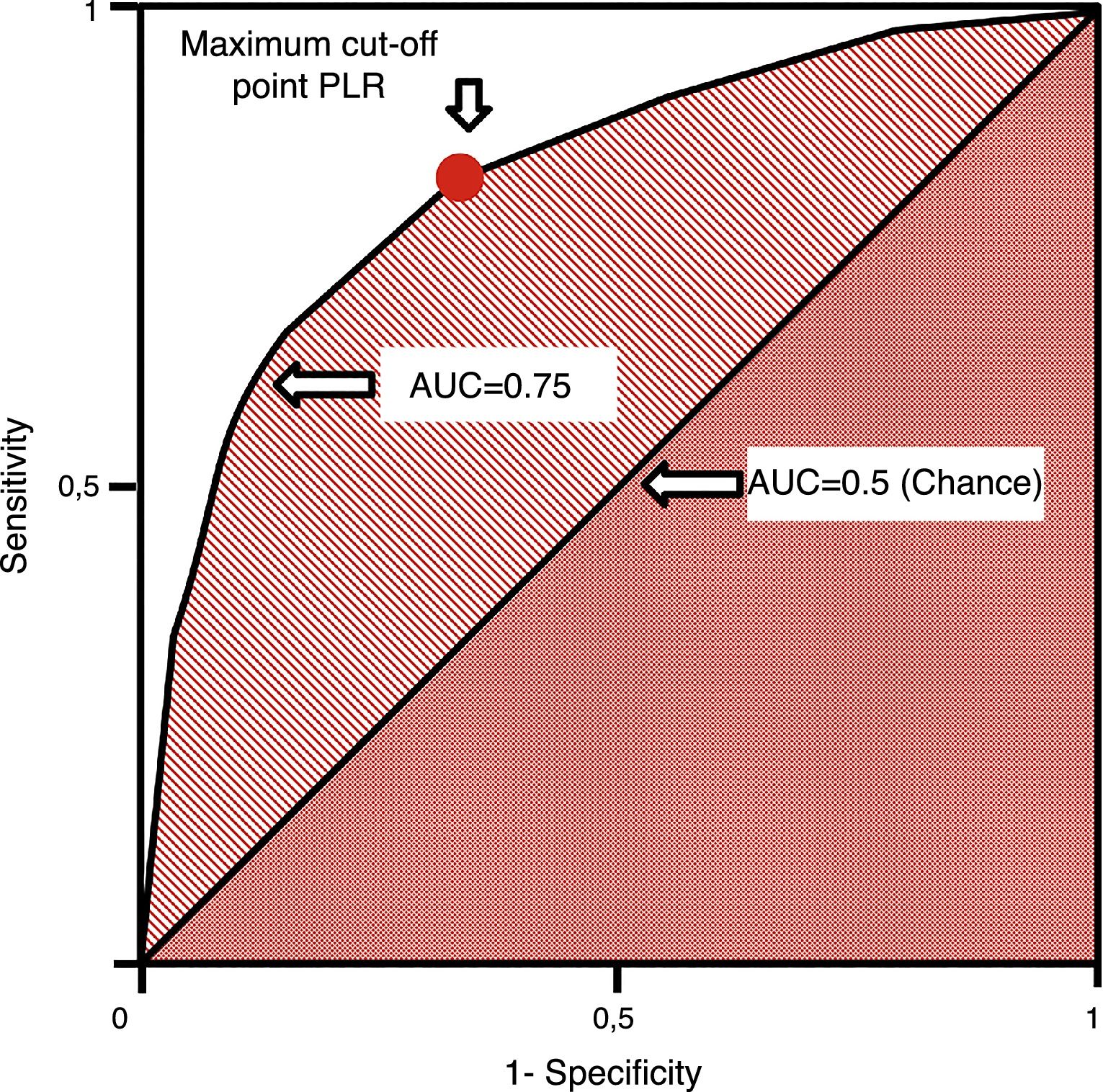
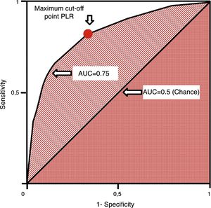
ROC (receiver operating characteristics) curves are used in quantitative tests and we can assign one diagnostic sensitivity and specificity likelihood ratio to every value or interval of results. This allows us to build one curve with pairs of diagnostic sensitivity and 1−specificity which is equivalent to positive likelihood ratios.37 They are measured using the area under the curve (AUC). The AUC is interpreted as the probability that by randomly selecting one sick individual and one healthy individual, the sick one has diagnostic value compared to the healthy one. The diagonal of the curve represents an AUC of 0.5 with a 50% chance that the classification is correct, which is equivalent to a random occurrence scenario. Thus, the closer the ROC curve comes to the diagonal, the more indicative it is of a low-value diagnostic test. ROC curves establish the cut-off point of maximum sensitivity and specificity for a given test (Fig. 4). Also, the AUCs can be compared using non-parametric tests such as the DeLong test.
ConclusionsStatistical tools should improve our capacity to understand the biological reality and the results that our interventions generate. Their adequate use and interpretation are essential to improve our patients’ health.
Conflicts of interestThe authors declare no conflicts of interest associated with this manuscript whatsoever.
Please cite this article as: García Garmendia JL, Maroto Monserrat F. Interpretación de resultados estadísticos. Med Intensiva. 2018;42:370–379.

